Note
Click here to download the full example code
Support recovery on MEG data
This example compares several methods that recover the support in the MEG/EEG source localization problem with statistical guarantees. Here we work with two datasets that study three different tasks (visual, audio, somato).
We reproduce the real data experiment of Chevalier et al. (2020) 1, which shows the benefit of (ensemble) clustered inference such as (ensemble of) clustered desparsified Multi-Task Lasso ((e)cd-MTLasso) over standard approach such as sLORETA. Specifically, it retrieves the support using a natural threshold (not computed a posteriori) of the estimated parameter. The estimated support enjoys statistical guarantees.
References
- 1
Chevalier, J. A., Gramfort, A., Salmon, J., & Thirion, B. (2020). Statistical control for spatio-temporal MEG/EEG source imaging with desparsified multi-task Lasso. In NeurIPS 2020-34h Conference on Neural Information Processing Systems.
import os
import numpy as np
import matplotlib.image as mpimg
import matplotlib.pyplot as plt
import mne
from scipy.sparse.csgraph import connected_components
from mne.datasets import sample, somato
from mne.inverse_sparse.mxne_inverse import _prepare_gain, _make_sparse_stc
from mne.minimum_norm import make_inverse_operator, apply_inverse
from sklearn.cluster import FeatureAgglomeration
from sklearn.metrics.pairwise import pairwise_distances

from hidimstat.clustered_inference import clustered_inference
from hidimstat.ensemble_clustered_inference import \
    ensemble_clustered_inference
from hidimstat.stat_tools import zscore_from_pval
Specific preprocessing functions
The functions below are used to load or preprocess the data or to put the solution in a convenient format. If you are reading this example for the first time, you should skip this section.
The following function loads the data from the sample dataset.
def _load_sample(cond):
    '''Load data from the sample dataset'''

    # Get data paths
    subject = 'sample'
    data_path = sample.data_path()
    fwd_fname_suffix = 'MEG/sample/sample_audvis-meg-eeg-oct-6-fwd.fif'
    fwd_fname = os.path.join(data_path, fwd_fname_suffix)
    ave_fname = os.path.join(data_path, 'MEG/sample/sample_audvis-ave.fif')
    cov_fname_suffix = 'MEG/sample/sample_audvis-shrunk-cov.fif'
    cov_fname = os.path.join(data_path, cov_fname_suffix)
    cov_fname = data_path + '/' + cov_fname_suffix
    subjects_dir = os.path.join(data_path, 'subjects')

    if cond == 'audio':
        condition = 'Left Auditory'
    elif cond == 'visual':
        condition = 'Left visual'

    # Read noise covariance matrix
    noise_cov = mne.read_cov(cov_fname)

    # Read forward matrix
    forward = mne.read_forward_solution(fwd_fname)

    # Handling average file
    evoked = mne.read_evokeds(ave_fname, condition=condition,
                              baseline=(None, 0))
    evoked = evoked.pick_types('grad')

    # Selecting relevant time window
    evoked.plot()
    t_min, t_max = 0.05, 0.1
    t_step = 0.01

    pca = False

    return (subject, subjects_dir, noise_cov, forward, evoked,
            t_min, t_max, t_step, pca)
The next function loads the data from the somato dataset.
def _load_somato(cond):
    '''Load data from the somato dataset'''

    # Get data paths
    data_path = somato.data_path()
    subject = '01'
    subjects_dir = data_path + '/derivatives/freesurfer/subjects'
    raw_fname = os.path.join(data_path, f'sub-{subject}', 'meg',
                             f'sub-{subject}_task-{cond}_meg.fif')
    fwd_fname = os.path.join(data_path, 'derivatives', f'sub-{subject}',
                             f'sub-{subject}_task-{cond}-fwd.fif')

    # Read evoked
    raw = mne.io.read_raw_fif(raw_fname)
    events = mne.find_events(raw, stim_channel='STI 014')
    reject = dict(grad=4000e-13, eog=350e-6)
    picks = mne.pick_types(raw.info, meg=True, eeg=True, eog=True)

    event_id, tmin, tmax = 1, -.2, .25
    epochs = mne.Epochs(raw, events, event_id, tmin, tmax, picks=picks,
                        reject=reject, preload=True)
    evoked = epochs.average()
    evoked = evoked.pick_types('grad')
    # evoked.plot()

    # Compute noise covariance matrix
    noise_cov = mne.compute_covariance(epochs, rank='info', tmax=0.)

    # Read forward matrix
    forward = mne.read_forward_solution(fwd_fname)

    # Selecting relevant time window: focusing on early signal
    t_min, t_max = 0.03, 0.05
    t_step = 1.0 / 300

    # We must reduce the whitener since data were preprocessed for removal
    # of environmental noise with maxwell filter leading to an effective
    # number of 64 samples.
    pca = True

    return (subject, subjects_dir, noise_cov, forward, evoked,
            t_min, t_max, t_step, pca)
The function below preprocess the raw M/EEG data, it notably computes the whitened MEG/EEG measurements and prepares the gain matrix.
def preprocess_meg_eeg_data(evoked, forward, noise_cov, loose=0., depth=0.,
                            pca=False):
    """Preprocess MEG or EEG data to produce the whitened MEG/EEG measurements
    (target) and the preprocessed gain matrix (design matrix). This function
    is mainly wrapping the `_prepare_gain` MNE function.

    Parameters
    ----------
    evoked : instance of mne.Evoked
        The evoked data.

    forward : instance of Forward
        The forward solution.

    noise_cov : instance of Covariance
        The noise covariance.

    loose : float in [0, 1] or 'auto'
        Value that weights the source variances of the dipole components
        that are parallel (tangential) to the cortical surface. If loose
        is 0 then the solution is computed with fixed orientation.
        If loose is 1, it corresponds to free orientations.
        The default value ('auto') is set to 0.2 for surface-oriented source
        space and set to 1.0 for volumic or discrete source space.
        See for details:
        https://mne.tools/stable/auto_tutorials/inverse/35_dipole_orientations.html?highlight=loose

    depth : None or float in [0, 1]
        Depth weighting coefficients. If None, no depth weighting is performed.

    pca : bool, optional (default=False)
        If True, whitener is reduced.
        If False, whitener is not reduced (square matrix).

    Returns
    -------
    G : array, shape (n_channels, n_dipoles)
        The preprocessed gain matrix. If pca=True then n_channels is
        effectively equal to the rank of the data.

    M : array, shape (n_channels, n_times)
        The whitened MEG/EEG measurements. If pca=True then n_channels is
        effectively equal to the rank of the data.

    forward : instance of Forward
        The preprocessed forward solution.
    """

    all_ch_names = evoked.ch_names

    # Handle depth weighting and whitening (here is no weights)
    forward, G, gain_info, whitener, _, _ = \
        _prepare_gain(forward, evoked.info, noise_cov, pca=pca, depth=depth,
                      loose=loose, weights=None, weights_min=None, rank=None)

    # Select channels of interest
    sel = [all_ch_names.index(name) for name in gain_info['ch_names']]

    M = evoked.data[sel]
    M = np.dot(whitener, M)

    return G, M, forward
The next function translates the solution in a readable format for the MNE plotting functions that require a Source Time Course (STC) object.
def _compute_stc(zscore_active_set, active_set, evoked, forward):
    """Wrapper of `_make_sparse_stc`"""

    X = np.atleast_2d(zscore_active_set)

    if X.shape[1] > 1 and X.shape[0] == 1:
        X = X.T

    stc = _make_sparse_stc(X, active_set, forward, tmin=evoked.times[0],
                           tstep=1. / evoked.info['sfreq'])
    return stc
The function below will be used to modify the connectivity matrix to avoid multiple warnings when we run the clustering algorithm.
def _fix_connectivity(X, connectivity, affinity):
    """Complete the connectivity matrix if necessary"""

    # Convert connectivity matrix into LIL format
    connectivity = connectivity.tolil()

    # Compute the number of nodes
    n_connected_components, labels = connected_components(connectivity)

    if n_connected_components > 1:

        for i in range(n_connected_components):
            idx_i = np.where(labels == i)[0]
            Xi = X[idx_i]
            for j in range(i):
                idx_j = np.where(labels == j)[0]
                Xj = X[idx_j]
                D = pairwise_distances(Xi, Xj, metric=affinity)
                ii, jj = np.where(D == np.min(D))
                ii = ii[0]
                jj = jj[0]
                connectivity[idx_i[ii], idx_j[jj]] = True
                connectivity[idx_j[jj], idx_i[ii]] = True

    return connectivity, n_connected_components
Downloading data
After choosing a task, we run the function that loads the data to get the corresponding evoked, forward and noise covariance matrices.
# Choose the experiment (task)
list_cond = ['audio', 'visual', 'somato']
cond = list_cond[2]
print(f"Let's process the condition: {cond}")

# Load the data
if cond in ['audio', 'visual']:
    sub, subs_dir, noise_cov, forward, evoked, t_min, t_max, t_step, pca = \
        _load_sample(cond)

elif cond == 'somato':
    sub, subs_dir, noise_cov, forward, evoked, t_min, t_max, t_step, pca = \
        _load_somato(cond)
Out:
Let's process the condition: somato
Using default location ~/mne_data for somato...
Creating ~/mne_data
Downloading archive MNE-somato-data.tar.gz to /home/runner/mne_data
Downloading https://files.osf.io/v1/resources/rxvq7/providers/osfstorage/59c0e2849ad5a1025d4b7346?version=7&action=download&direct (582.2 MB)

  0%|          | Downloading : 0.00/582M [00:00<?,        ?B/s]
  0%|          | Downloading : 0.99M/582M [00:00<00:25,    24.2MB/s]
  0%|          | Downloading : 2.49M/582M [00:00<00:24,    25.0MB/s]
  1%|          | Downloading : 4.49M/582M [00:00<00:23,    25.9MB/s]
  1%|1         | Downloading : 6.49M/582M [00:00<00:22,    26.9MB/s]
  2%|1         | Downloading : 10.5M/582M [00:00<00:21,    28.0MB/s]
  2%|2         | Downloading : 14.5M/582M [00:00<00:20,    29.1MB/s]
  3%|3         | Downloading : 18.5M/582M [00:00<00:19,    30.3MB/s]
  4%|3         | Downloading : 20.5M/582M [00:00<00:18,    31.5MB/s]
  4%|3         | Downloading : 22.5M/582M [00:00<00:17,    32.7MB/s]
  4%|4         | Downloading : 24.5M/582M [00:00<00:17,    33.8MB/s]
  5%|4         | Downloading : 26.5M/582M [00:00<00:16,    35.0MB/s]
  5%|4         | Downloading : 28.5M/582M [00:00<00:16,    36.3MB/s]
  5%|5         | Downloading : 30.5M/582M [00:00<00:15,    37.4MB/s]
  6%|5         | Downloading : 32.5M/582M [00:00<00:14,    38.6MB/s]
  6%|5         | Downloading : 34.5M/582M [00:00<00:14,    39.9MB/s]
  6%|6         | Downloading : 36.5M/582M [00:00<00:13,    41.2MB/s]
  7%|6         | Downloading : 38.5M/582M [00:00<00:13,    42.5MB/s]
  7%|6         | Downloading : 40.5M/582M [00:00<00:12,    43.9MB/s]
  7%|7         | Downloading : 42.5M/582M [00:00<00:12,    45.4MB/s]
  8%|7         | Downloading : 44.5M/582M [00:00<00:12,    46.8MB/s]
  8%|7         | Downloading : 46.5M/582M [00:00<00:11,    48.1MB/s]
  8%|8         | Downloading : 48.5M/582M [00:00<00:11,    49.4MB/s]
  9%|8         | Downloading : 50.5M/582M [00:00<00:11,    50.3MB/s]
  9%|9         | Downloading : 52.5M/582M [00:00<00:10,    51.8MB/s]
 10%|9         | Downloading : 56.5M/582M [00:00<00:10,    53.3MB/s]
 10%|#         | Downloading : 58.5M/582M [00:00<00:09,    54.9MB/s]
 10%|#         | Downloading : 60.5M/582M [00:00<00:09,    56.4MB/s]
 11%|#         | Downloading : 62.5M/582M [00:00<00:09,    57.5MB/s]
 11%|#1        | Downloading : 64.5M/582M [00:00<00:09,    58.9MB/s]
 11%|#1        | Downloading : 66.5M/582M [00:00<00:08,    60.5MB/s]
 12%|#2        | Downloading : 72.5M/582M [00:00<00:08,    62.2MB/s]
 13%|#3        | Downloading : 76.5M/582M [00:00<00:08,    63.5MB/s]
 14%|#3        | Downloading : 80.5M/582M [00:00<00:08,    65.7MB/s]
 15%|#4        | Downloading : 84.5M/582M [00:00<00:07,    67.3MB/s]
 15%|#5        | Downloading : 88.5M/582M [00:00<00:07,    68.2MB/s]
 16%|#5        | Downloading : 92.5M/582M [00:00<00:07,    70.3MB/s]
 17%|#6        | Downloading : 96.5M/582M [00:00<00:07,    72.2MB/s]
 17%|#7        | Downloading : 100M/582M [00:00<00:06,    73.7MB/s]
 18%|#7        | Downloading : 104M/582M [00:00<00:06,    74.7MB/s]
 19%|#8        | Downloading : 108M/582M [00:01<00:06,    74.8MB/s]
 19%|#9        | Downloading : 112M/582M [00:01<00:06,    72.1MB/s]
 20%|##        | Downloading : 116M/582M [00:01<00:08,    58.7MB/s]
 20%|##        | Downloading : 118M/582M [00:01<00:08,    59.4MB/s]
 21%|##        | Downloading : 120M/582M [00:01<00:08,    60.5MB/s]
 21%|##1       | Downloading : 122M/582M [00:01<00:07,    61.8MB/s]
 21%|##1       | Downloading : 124M/582M [00:01<00:07,    62.7MB/s]
 22%|##1       | Downloading : 126M/582M [00:01<00:07,    61.5MB/s]
 22%|##2       | Downloading : 128M/582M [00:01<00:07,    61.0MB/s]
 23%|##2       | Downloading : 132M/582M [00:01<00:07,    61.8MB/s]
 23%|##3       | Downloading : 134M/582M [00:01<00:07,    61.8MB/s]
 23%|##3       | Downloading : 136M/582M [00:01<00:07,    62.8MB/s]
 24%|##3       | Downloading : 138M/582M [00:01<00:07,    63.4MB/s]
 24%|##4       | Downloading : 140M/582M [00:01<00:07,    64.8MB/s]
 24%|##4       | Downloading : 142M/582M [00:01<00:07,    65.0MB/s]
 25%|##4       | Downloading : 144M/582M [00:01<00:07,    63.9MB/s]
 25%|##5       | Downloading : 146M/582M [00:01<00:07,    64.7MB/s]
 26%|##5       | Downloading : 148M/582M [00:01<00:06,    65.6MB/s]
 26%|##5       | Downloading : 150M/582M [00:01<00:06,    66.3MB/s]
 26%|##6       | Downloading : 152M/582M [00:01<00:06,    66.5MB/s]
 27%|##6       | Downloading : 154M/582M [00:02<00:06,    66.2MB/s]
 27%|##6       | Downloading : 156M/582M [00:02<00:06,    66.8MB/s]
 27%|##7       | Downloading : 158M/582M [00:02<00:06,    66.9MB/s]
 28%|##7       | Downloading : 162M/582M [00:02<00:06,    68.3MB/s]
 28%|##8       | Downloading : 164M/582M [00:02<00:06,    69.0MB/s]
 29%|##8       | Downloading : 166M/582M [00:02<00:06,    69.5MB/s]
 29%|##8       | Downloading : 168M/582M [00:02<00:06,    69.9MB/s]
 29%|##9       | Downloading : 170M/582M [00:02<00:06,    70.8MB/s]
 30%|##9       | Downloading : 172M/582M [00:02<00:05,    72.0MB/s]
 30%|##9       | Downloading : 174M/582M [00:02<00:05,    72.7MB/s]
 30%|###       | Downloading : 176M/582M [00:02<00:05,    72.9MB/s]
 31%|###       | Downloading : 178M/582M [00:02<00:05,    72.8MB/s]
 31%|###1      | Downloading : 180M/582M [00:02<00:05,    72.8MB/s]
 31%|###1      | Downloading : 182M/582M [00:02<00:05,    73.7MB/s]
 32%|###1      | Downloading : 184M/582M [00:02<00:05,    74.4MB/s]
 32%|###2      | Downloading : 186M/582M [00:02<00:05,    75.0MB/s]
 32%|###2      | Downloading : 188M/582M [00:02<00:06,    65.6MB/s]
 33%|###2      | Downloading : 191M/582M [00:02<00:06,    66.6MB/s]
 33%|###3      | Downloading : 193M/582M [00:02<00:06,    62.7MB/s]
 34%|###3      | Downloading : 195M/582M [00:02<00:06,    62.5MB/s]
 34%|###3      | Downloading : 197M/582M [00:02<00:06,    63.2MB/s]
 34%|###4      | Downloading : 199M/582M [00:02<00:06,    63.7MB/s]
 35%|###4      | Downloading : 201M/582M [00:02<00:06,    64.2MB/s]
 35%|###4      | Downloading : 203M/582M [00:02<00:06,    63.9MB/s]
 35%|###5      | Downloading : 205M/582M [00:02<00:06,    64.7MB/s]
 36%|###5      | Downloading : 207M/582M [00:02<00:05,    65.6MB/s]
 36%|###5      | Downloading : 209M/582M [00:02<00:05,    66.4MB/s]
 36%|###6      | Downloading : 211M/582M [00:02<00:05,    66.9MB/s]
 37%|###6      | Downloading : 213M/582M [00:02<00:05,    67.4MB/s]
 37%|###7      | Downloading : 215M/582M [00:02<00:05,    68.9MB/s]
 37%|###7      | Downloading : 217M/582M [00:02<00:05,    69.8MB/s]
 38%|###7      | Downloading : 219M/582M [00:02<00:05,    70.8MB/s]
 38%|###8      | Downloading : 221M/582M [00:02<00:05,    71.4MB/s]
 38%|###8      | Downloading : 223M/582M [00:02<00:05,    72.7MB/s]
 39%|###8      | Downloading : 225M/582M [00:03<00:05,    73.5MB/s]
 39%|###9      | Downloading : 227M/582M [00:03<00:05,    74.3MB/s]
 39%|###9      | Downloading : 229M/582M [00:03<00:04,    75.7MB/s]
 40%|###9      | Downloading : 231M/582M [00:03<00:04,    76.0MB/s]
 40%|####      | Downloading : 233M/582M [00:03<00:04,    76.7MB/s]
 40%|####      | Downloading : 235M/582M [00:03<00:04,    76.8MB/s]
 41%|####      | Downloading : 237M/582M [00:03<00:04,    75.3MB/s]
 41%|####1     | Downloading : 239M/582M [00:03<00:04,    76.1MB/s]
 41%|####1     | Downloading : 241M/582M [00:03<00:04,    75.6MB/s]
 42%|####1     | Downloading : 243M/582M [00:03<00:04,    71.2MB/s]
 42%|####2     | Downloading : 245M/582M [00:03<00:04,    71.4MB/s]
 43%|####2     | Downloading : 247M/582M [00:03<00:04,    72.2MB/s]
 43%|####2     | Downloading : 249M/582M [00:03<00:04,    72.7MB/s]
 43%|####3     | Downloading : 251M/582M [00:03<00:04,    72.1MB/s]
 44%|####3     | Downloading : 253M/582M [00:03<00:04,    73.4MB/s]
 44%|####3     | Downloading : 255M/582M [00:03<00:04,    73.1MB/s]
 44%|####4     | Downloading : 257M/582M [00:03<00:04,    73.9MB/s]
 45%|####4     | Downloading : 259M/582M [00:03<00:04,    75.2MB/s]
 45%|####4     | Downloading : 261M/582M [00:03<00:04,    75.7MB/s]
 45%|####5     | Downloading : 263M/582M [00:03<00:04,    76.7MB/s]
 46%|####5     | Downloading : 265M/582M [00:03<00:04,    77.8MB/s]
 46%|####5     | Downloading : 267M/582M [00:03<00:04,    77.3MB/s]
 46%|####6     | Downloading : 269M/582M [00:03<00:04,    78.6MB/s]
 47%|####6     | Downloading : 271M/582M [00:03<00:04,    78.9MB/s]
 47%|####6     | Downloading : 273M/582M [00:03<00:04,    67.9MB/s]
 47%|####7     | Downloading : 274M/582M [00:03<00:06,    53.7MB/s]
 47%|####7     | Downloading : 275M/582M [00:03<00:06,    52.8MB/s]
 47%|####7     | Downloading : 276M/582M [00:03<00:06,    52.1MB/s]
 48%|####7     | Downloading : 277M/582M [00:03<00:06,    51.5MB/s]
 48%|####7     | Downloading : 278M/582M [00:03<00:06,    51.6MB/s]
 48%|####8     | Downloading : 279M/582M [00:03<00:06,    51.6MB/s]
 48%|####8     | Downloading : 280M/582M [00:03<00:06,    52.1MB/s]
 48%|####8     | Downloading : 281M/582M [00:03<00:06,    52.4MB/s]
 49%|####8     | Downloading : 284M/582M [00:04<00:05,    53.6MB/s]
 49%|####9     | Downloading : 286M/582M [00:04<00:05,    54.8MB/s]
 50%|####9     | Downloading : 288M/582M [00:04<00:05,    55.5MB/s]
 50%|####9     | Downloading : 290M/582M [00:04<00:05,    56.5MB/s]
 50%|#####     | Downloading : 292M/582M [00:04<00:05,    57.5MB/s]
 51%|#####     | Downloading : 294M/582M [00:04<00:05,    58.1MB/s]
 51%|#####     | Downloading : 296M/582M [00:04<00:05,    59.2MB/s]
 51%|#####1    | Downloading : 298M/582M [00:04<00:04,    60.0MB/s]
 52%|#####1    | Downloading : 300M/582M [00:04<00:04,    61.5MB/s]
 52%|#####1    | Downloading : 302M/582M [00:04<00:04,    62.7MB/s]
 52%|#####2    | Downloading : 304M/582M [00:04<00:04,    63.7MB/s]
 53%|#####2    | Downloading : 306M/582M [00:04<00:04,    64.7MB/s]
 53%|#####2    | Downloading : 308M/582M [00:04<00:04,    65.4MB/s]
 53%|#####3    | Downloading : 310M/582M [00:04<00:04,    66.9MB/s]
 54%|#####3    | Downloading : 312M/582M [00:04<00:04,    68.2MB/s]
 54%|#####4    | Downloading : 314M/582M [00:04<00:04,    69.6MB/s]
 54%|#####4    | Downloading : 316M/582M [00:04<00:03,    70.8MB/s]
 55%|#####4    | Downloading : 318M/582M [00:04<00:03,    70.8MB/s]
 55%|#####5    | Downloading : 320M/582M [00:04<00:03,    69.2MB/s]
 56%|#####5    | Downloading : 324M/582M [00:04<00:03,    69.0MB/s]
 57%|#####6    | Downloading : 330M/582M [00:04<00:03,    70.6MB/s]
 57%|#####7    | Downloading : 334M/582M [00:04<00:03,    71.0MB/s]
 58%|#####8    | Downloading : 338M/582M [00:04<00:03,    71.9MB/s]
 59%|#####8    | Downloading : 342M/582M [00:04<00:03,    72.7MB/s]
 60%|#####9    | Downloading : 346M/582M [00:04<00:03,    73.5MB/s]
 60%|######    | Downloading : 350M/582M [00:04<00:03,    74.9MB/s]
 61%|######    | Downloading : 354M/582M [00:04<00:03,    74.4MB/s]
 62%|######1   | Downloading : 358M/582M [00:04<00:03,    71.6MB/s]
 62%|######2   | Downloading : 362M/582M [00:05<00:03,    68.8MB/s]
 63%|######2   | Downloading : 364M/582M [00:05<00:03,    57.5MB/s]
 63%|######2   | Downloading : 366M/582M [00:05<00:03,    57.0MB/s]
 63%|######3   | Downloading : 369M/582M [00:05<00:03,    58.2MB/s]
 64%|######3   | Downloading : 371M/582M [00:05<00:03,    58.8MB/s]
 64%|######4   | Downloading : 373M/582M [00:05<00:03,    59.0MB/s]
 64%|######4   | Downloading : 375M/582M [00:05<00:03,    60.4MB/s]
 65%|######4   | Downloading : 377M/582M [00:05<00:03,    61.2MB/s]
 65%|######5   | Downloading : 379M/582M [00:05<00:03,    61.5MB/s]
 66%|######5   | Downloading : 381M/582M [00:05<00:03,    62.6MB/s]
 66%|######5   | Downloading : 383M/582M [00:05<00:03,    63.3MB/s]
 66%|######6   | Downloading : 385M/582M [00:05<00:03,    64.1MB/s]
 67%|######6   | Downloading : 387M/582M [00:05<00:03,    65.1MB/s]
 67%|######6   | Downloading : 389M/582M [00:05<00:03,    65.3MB/s]
 67%|######7   | Downloading : 391M/582M [00:05<00:03,    66.3MB/s]
 68%|######7   | Downloading : 393M/582M [00:05<00:02,    67.3MB/s]
 68%|######7   | Downloading : 395M/582M [00:05<00:02,    68.6MB/s]
 68%|######8   | Downloading : 397M/582M [00:05<00:02,    70.2MB/s]
 69%|######8   | Downloading : 399M/582M [00:05<00:02,    71.3MB/s]
 69%|######8   | Downloading : 401M/582M [00:05<00:02,    72.3MB/s]
 69%|######9   | Downloading : 403M/582M [00:05<00:02,    73.5MB/s]
 70%|######9   | Downloading : 407M/582M [00:05<00:02,    74.9MB/s]
 70%|#######   | Downloading : 409M/582M [00:05<00:02,    76.2MB/s]
 71%|#######   | Downloading : 411M/582M [00:05<00:02,    77.3MB/s]
 71%|#######1  | Downloading : 413M/582M [00:05<00:02,    78.1MB/s]
 71%|#######1  | Downloading : 415M/582M [00:05<00:02,    79.4MB/s]
 72%|#######1  | Downloading : 417M/582M [00:05<00:02,    79.9MB/s]
 72%|#######2  | Downloading : 419M/582M [00:05<00:02,    78.1MB/s]
 72%|#######2  | Downloading : 421M/582M [00:05<00:02,    79.0MB/s]
 73%|#######2  | Downloading : 423M/582M [00:05<00:02,    79.3MB/s]
 73%|#######3  | Downloading : 425M/582M [00:05<00:02,    79.0MB/s]
 73%|#######3  | Downloading : 427M/582M [00:05<00:02,    79.0MB/s]
 74%|#######3  | Downloading : 429M/582M [00:05<00:02,    79.3MB/s]
 74%|#######4  | Downloading : 431M/582M [00:06<00:02,    78.6MB/s]
 74%|#######4  | Downloading : 433M/582M [00:06<00:01,    79.8MB/s]
 75%|#######4  | Downloading : 435M/582M [00:06<00:01,    80.6MB/s]
 75%|#######5  | Downloading : 437M/582M [00:06<00:01,    81.7MB/s]
 75%|#######5  | Downloading : 439M/582M [00:06<00:01,    83.0MB/s]
 76%|#######5  | Downloading : 441M/582M [00:06<00:01,    84.2MB/s]
 76%|#######6  | Downloading : 443M/582M [00:06<00:01,    85.0MB/s]
 77%|#######6  | Downloading : 445M/582M [00:06<00:01,    85.7MB/s]
 77%|#######6  | Downloading : 447M/582M [00:06<00:01,    85.8MB/s]
 78%|#######7  | Downloading : 451M/582M [00:06<00:01,    82.4MB/s]
 78%|#######7  | Downloading : 453M/582M [00:06<00:02,    65.7MB/s]
 78%|#######8  | Downloading : 454M/582M [00:06<00:02,    65.0MB/s]
 78%|#######8  | Downloading : 456M/582M [00:06<00:02,    64.6MB/s]
 79%|#######8  | Downloading : 459M/582M [00:06<00:01,    65.2MB/s]
 79%|#######9  | Downloading : 461M/582M [00:06<00:01,    66.4MB/s]
 80%|#######9  | Downloading : 463M/582M [00:06<00:01,    67.5MB/s]
 80%|#######9  | Downloading : 465M/582M [00:06<00:01,    68.9MB/s]
 80%|########  | Downloading : 467M/582M [00:06<00:01,    69.4MB/s]
 81%|########  | Downloading : 469M/582M [00:06<00:01,    69.5MB/s]
 81%|########  | Downloading : 471M/582M [00:06<00:01,    70.6MB/s]
 81%|########1 | Downloading : 473M/582M [00:06<00:01,    71.8MB/s]
 82%|########1 | Downloading : 475M/582M [00:06<00:01,    73.0MB/s]
 82%|########2 | Downloading : 477M/582M [00:06<00:01,    74.3MB/s]
 82%|########2 | Downloading : 479M/582M [00:06<00:01,    75.4MB/s]
 83%|########2 | Downloading : 481M/582M [00:06<00:01,    76.1MB/s]
 83%|########3 | Downloading : 483M/582M [00:06<00:01,    77.0MB/s]
 83%|########3 | Downloading : 485M/582M [00:06<00:01,    77.7MB/s]
 84%|########3 | Downloading : 487M/582M [00:06<00:01,    78.6MB/s]
 84%|########4 | Downloading : 489M/582M [00:06<00:01,    79.7MB/s]
 84%|########4 | Downloading : 491M/582M [00:06<00:01,    81.0MB/s]
 85%|########4 | Downloading : 493M/582M [00:06<00:01,    81.5MB/s]
 85%|########5 | Downloading : 495M/582M [00:06<00:01,    79.7MB/s]
 85%|########5 | Downloading : 497M/582M [00:06<00:01,    79.9MB/s]
 86%|########5 | Downloading : 499M/582M [00:06<00:01,    79.6MB/s]
 86%|########6 | Downloading : 501M/582M [00:06<00:01,    80.3MB/s]
 86%|########6 | Downloading : 503M/582M [00:07<00:01,    79.8MB/s]
 87%|########6 | Downloading : 505M/582M [00:07<00:01,    79.6MB/s]
 87%|########7 | Downloading : 507M/582M [00:07<00:00,    79.7MB/s]
 88%|########7 | Downloading : 509M/582M [00:07<00:00,    79.6MB/s]
 88%|########7 | Downloading : 511M/582M [00:07<00:00,    79.2MB/s]
 88%|########8 | Downloading : 513M/582M [00:07<00:00,    79.1MB/s]
 89%|########8 | Downloading : 515M/582M [00:07<00:00,    74.9MB/s]
 89%|########8 | Downloading : 517M/582M [00:07<00:00,    74.7MB/s]
 89%|########9 | Downloading : 519M/582M [00:07<00:00,    75.0MB/s]
 90%|########9 | Downloading : 521M/582M [00:07<00:00,    74.9MB/s]
 90%|########9 | Downloading : 523M/582M [00:07<00:00,    75.9MB/s]
 90%|######### | Downloading : 525M/582M [00:07<00:00,    75.7MB/s]
 91%|######### | Downloading : 527M/582M [00:07<00:00,    74.7MB/s]
 92%|#########1| Downloading : 533M/582M [00:07<00:00,    74.6MB/s]
 92%|#########2| Downloading : 537M/582M [00:07<00:00,    74.0MB/s]
 93%|#########3| Downloading : 541M/582M [00:07<00:00,    68.7MB/s]
 93%|#########3| Downloading : 543M/582M [00:07<00:00,    70.2MB/s]
 94%|#########3| Downloading : 545M/582M [00:07<00:00,    71.6MB/s]
 94%|#########4| Downloading : 547M/582M [00:07<00:00,    72.7MB/s]
 94%|#########4| Downloading : 549M/582M [00:07<00:00,    74.3MB/s]
 95%|#########4| Downloading : 551M/582M [00:07<00:00,    75.8MB/s]
 95%|#########5| Downloading : 553M/582M [00:07<00:00,    76.6MB/s]
 95%|#########5| Downloading : 555M/582M [00:07<00:00,    77.4MB/s]
 96%|#########6| Downloading : 559M/582M [00:07<00:00,    78.8MB/s]
 97%|#########6| Downloading : 563M/582M [00:07<00:00,    80.4MB/s]
 97%|#########7| Downloading : 565M/582M [00:07<00:00,    80.9MB/s]
 97%|#########7| Downloading : 567M/582M [00:07<00:00,    80.6MB/s]
 98%|#########7| Downloading : 569M/582M [00:07<00:00,    80.5MB/s]
 98%|#########8| Downloading : 571M/582M [00:07<00:00,    79.6MB/s]
 99%|#########8| Downloading : 573M/582M [00:08<00:00,    79.7MB/s]
 99%|#########8| Downloading : 575M/582M [00:08<00:00,    80.5MB/s]
 99%|#########9| Downloading : 577M/582M [00:08<00:00,    82.0MB/s]
100%|#########9| Downloading : 579M/582M [00:08<00:00,    83.2MB/s]
100%|#########9| Downloading : 581M/582M [00:08<00:00,    84.7MB/s]
100%|##########| Downloading : 582M/582M [00:08<00:00,    75.4MB/s]
Verifying hash 32fd2f6c8c7eb0784a1de6435273c48b.
Decompressing the archive: /home/runner/mne_data/MNE-somato-data.tar.gz
(please be patient, this can take some time)
Successfully extracted to: ['/home/runner/mne_data/MNE-somato-data']
Attempting to create new mne-python configuration file:
/home/runner/.mne/mne-python.json
Opening raw data file /home/runner/mne_data/MNE-somato-data/sub-01/meg/sub-01_task-somato_meg.fif...
    Range : 237600 ... 506999 =    791.189 ...  1688.266 secs
Ready.
111 events found
Event IDs: [1]
Not setting metadata
Not setting metadata
111 matching events found
Setting baseline interval to [-0.19979521315838786, 0.0] sec
Applying baseline correction (mode: mean)
0 projection items activated
Loading data for 111 events and 136 original time points ...
0 bad epochs dropped
Computing rank from data with rank='info'
    MEG: rank 64 after 0 projectors applied to 306 channels
    Setting small MEG eigenvalues to zero (without PCA)
Reducing data rank from 306 -> 64
Estimating covariance using EMPIRICAL
Done.
Number of samples used : 6771
[done]
Reading forward solution from /home/runner/mne_data/MNE-somato-data/derivatives/sub-01/sub-01_task-somato-fwd.fif...
    Reading a source space...
    [done]
    Reading a source space...
    [done]
    2 source spaces read
    Desired named matrix (kind = 3523) not available
    Read MEG forward solution (8155 sources, 306 channels, free orientations)
    Source spaces transformed to the forward solution coordinate frame
Preparing data for clustered inference
For clustered inference we need the targets Y, the design matrix X
and the connectivity matrix, which is a sparse adjacency matrix.
# Collecting features' connectivity
connectivity = mne.source_estimate.spatial_src_adjacency(forward['src'])

# Croping evoked according to relevant time window
evoked.crop(tmin=t_min, tmax=t_max)

# Choosing frequency and number of clusters used for compression.
# Reducing the frequency to 100Hz to make inference faster
step = int(t_step * evoked.info['sfreq'])
evoked.decimate(step)
t_min = evoked.times[0]
t_step = 1. / evoked.info['sfreq']

# Preprocessing MEG data
X, Y, forward = preprocess_meg_eeg_data(evoked, forward, noise_cov, pca=pca)
Out:
-- number of adjacent vertices : 8196
/home/runner/work/hidimstat/hidimstat/examples/plot_meg_data_example.py:289: RuntimeWarning: 0.5% of original source space vertices have been omitted, tri-based adjacency will have holes.
Consider using distance-based adjacency or morphing data to all source space vertices.
  connectivity = mne.source_estimate.spatial_src_adjacency(forward['src'])
Converting forward solution to fixed orietnation
    No patch info available. The standard source space normals will be employed in the rotation to the local surface coordinates....
    Changing to fixed-orientation forward solution with surface-based source orientations...
    [done]
Computing inverse operator with 204 channels.
    204 out of 306 channels remain after picking
Selected 204 channels
Whitening the forward solution.
Computing rank from covariance with rank=None
    Using tolerance 2.1e-12 (2.2e-16 eps * 204 dim * 46  max singular value)
    Estimated rank (grad): 64
    GRAD: rank 64 computed from 204 data channels with 0 projectors
    Setting small GRAD eigenvalues to zero (without PCA)
Creating the source covariance matrix
Adjusting source covariance matrix.
Running clustered inference
For MEG data n_clusters = 1000 is generally a good default choice.
Taking n_clusters > 2000 might lead to an unpowerful inference.
Taking n_clusters < 500 might compress too much the data leading
to a compressed problem not close enough to the original problem.
n_clusters = 1000

# Setting theoretical FWER target
fwer_target = 0.1

# Computing threshold taking into account for Bonferroni correction
correction_clust_inf = 1. / n_clusters
zscore_threshold = zscore_from_pval((fwer_target / 2) * correction_clust_inf)

# Initializing FeatureAgglomeration object used for the clustering step
connectivity_fixed, _ = \
    _fix_connectivity(X.T, connectivity, affinity="euclidean")
ward = FeatureAgglomeration(n_clusters=n_clusters, connectivity=connectivity)

# Making the inference with the clustered inference algorithm
inference_method = 'desparsified-group-lasso'
beta_hat, pval, pval_corr, one_minus_pval, one_minus_pval_corr = \
    clustered_inference(X, Y, ward, n_clusters, method=inference_method)

# Extracting active set (support)
active_set = np.logical_or(pval_corr < fwer_target / 2,
                           one_minus_pval_corr < fwer_target / 2)
active_set_full = np.copy(active_set)
active_set_full[:] = True

# Translating p-vals into z-scores for nicer visualization
zscore = zscore_from_pval(pval, one_minus_pval)
zscore_active_set = zscore[active_set]
Out:
Clustered inference: n_clusters = 1000, inference method = desparsified-group-lasso, seed = 0
/home/runner/.local/lib/python3.8/site-packages/sklearn/cluster/_agglomerative.py:245: UserWarning: the number of connected components of the connectivity matrix is 2 > 1. Completing it to avoid stopping the tree early.
  connectivity, n_connected_components = _fix_connectivity(
/home/runner/work/hidimstat/hidimstat/hidimstat/desparsified_lasso.py:32: VisibleDeprecationWarning: Creating an ndarray from ragged nested sequences (which is a list-or-tuple of lists-or-tuples-or ndarrays with different lengths or shapes) is deprecated. If you meant to do this, you must specify 'dtype=object' when creating the ndarray.
  results = np.asarray(results)
Group reid: AR1 cov estimation
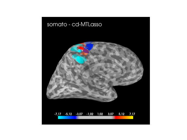
Visualization
Now, let us plot the thresholded statistical maps derived thanks to the clustered inference algorithm referred as cd-MTLasso.
# Let's put the solution into the format supported by the plotting functions
stc = _compute_stc(zscore_active_set, active_set, evoked, forward)

# Plotting parameters
if cond == 'audio':
    hemi = 'lh'
    view = 'lateral'
elif cond == 'visual':
    hemi = 'rh'
    view = 'medial'
elif cond == 'somato':
    hemi = 'rh'
    view = 'lateral'

# Plotting clustered inference solution
mne.viz.set_3d_backend("pyvista")

if active_set.sum() != 0:
    max_stc = np.max(np.abs(stc.data))
    clim = dict(pos_lims=(3, zscore_threshold, max_stc), kind='value')
    brain = stc.plot(subject=sub, hemi=hemi, clim=clim, subjects_dir=subs_dir,
                     views=view, time_viewer=False)
    brain.add_text(0.05, 0.9, f'{cond} - cd-MTLasso', 'title',
                   font_size=20)

# Hack for nice figures on HiDimStat website
save_fig = False
plot_saved_fig = True
if save_fig:
    brain.save_image(f'figures/meg_{cond}_cd-MTLasso.png')
if plot_saved_fig:
    brain.close()
    img = mpimg.imread(f'figures/meg_{cond}_cd-MTLasso.png')
    plt.imshow(img)
    plt.axis('off')
    plt.show()

interactive_plot = False
if interactive_plot:
    brain = \
        stc.plot(subject=sub, hemi='both', subjects_dir=subs_dir, clim=clim)
Out:
Using pyvista 3d backend.

/home/runner/.local/lib/python3.8/site-packages/pyvista/core/dataset.py:1192: PyvistaDeprecationWarning: Use of `point_arrays` is deprecated. Use `point_data` instead.
  warnings.warn(
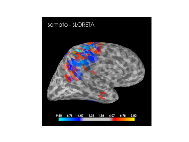
Comparision with sLORETA
Now, we compare the results derived from cd-MTLasso with the solution obtained from the one of the most standard approach: sLORETA.
# Running sLORETA with standard hyper-parameter
lambda2 = 1. / 9
inv = make_inverse_operator(evoked.info, forward, noise_cov, loose=0.,
                            depth=0., fixed=True)
stc_full = apply_inverse(evoked, inv, lambda2=lambda2, method='sLORETA')
stc_full = stc_full.mean()

# Computing threshold taking into account for Bonferroni correction
n_features = stc_full.data.size
correction = 1. / n_features
zscore_threshold_no_clust = zscore_from_pval((fwer_target / 2) * correction)

# Computing estimated support by sLORETA
active_set = np.abs(stc_full.data) > zscore_threshold_no_clust
active_set = active_set.flatten()

# Putting the solution into the format supported by the plotting functions
sLORETA_solution = np.atleast_2d(stc_full.data[active_set]).flatten()
stc = _make_sparse_stc(sLORETA_solution, active_set, forward, stc_full.tmin,
                       tstep=stc_full.tstep)

# Plotting sLORETA solution
if active_set.sum() != 0:
    max_stc = np.max(np.abs(stc.data))
    clim = dict(pos_lims=(3, zscore_threshold_no_clust, max_stc), kind='value')
    brain = stc.plot(subject=sub, hemi=hemi, clim=clim, subjects_dir=subs_dir,
                     views=view, time_viewer=False)
    brain.add_text(0.05, 0.9, f'{cond} - sLORETA', 'title', font_size=20)

    # Hack for nice figures on HiDimStat website
    if save_fig:
        brain.save_image(f'figures/meg_{cond}_sLORETA.png')
    if plot_saved_fig:
        brain.close()
        img = mpimg.imread(f'figures/meg_{cond}_sLORETA.png')
        plt.imshow(img)
        plt.axis('off')
        plt.show()
Out:
Computing inverse operator with 204 channels.
    204 out of 204 channels remain after picking
Selected 204 channels
Whitening the forward solution.
Computing rank from covariance with rank=None
    Using tolerance 2.1e-12 (2.2e-16 eps * 204 dim * 46  max singular value)
    Estimated rank (grad): 64
    GRAD: rank 64 computed from 204 data channels with 0 projectors
    Setting small GRAD eigenvalues to zero (without PCA)
Creating the source covariance matrix
Adjusting source covariance matrix.
Computing SVD of whitened and weighted lead field matrix.
    largest singular value = 2.06293
    scaling factor to adjust the trace = 2.84039e+19 (nchan = 204 nzero = 140)
Preparing the inverse operator for use...
    Scaled noise and source covariance from nave = 1 to nave = 111
    Created the regularized inverter
    The projection vectors do not apply to these channels.
    Created the whitener using a noise covariance matrix with rank 64 (140 small eigenvalues omitted)
    Computing noise-normalization factors (sLORETA)...
[done]
Applying inverse operator to "1"...
    Picked 204 channels from the data
    Computing inverse...
    Eigenleads need to be weighted ...
    Computing residual...
    Explained  95.4% variance
    sLORETA...
[done]
/home/runner/.local/lib/python3.8/site-packages/pyvista/core/dataset.py:1192: PyvistaDeprecationWarning: Use of `point_arrays` is deprecated. Use `point_data` instead.
  warnings.warn(
Analysis of the results
While the clustered inference solution always highlights the expected cortex (audio, visual or somato-sensory) with a universal predertemined threshold, the solution derived from the sLORETA method does not enjoy the same property. For the audio task the method is conservative and for the somato task the method makes false discoveries (then it seems anti-conservative).
Running ensemble clustered inference
To go further it is possible to run the ensemble clustered inference
algorithm. It might take several minutes on standard device with
n_jobs=1 (around 10 min). Just set
run_ensemble_clustered_inference=True below.
run_ensemble_clustered_inference = False

if run_ensemble_clustered_inference:
    # Making the inference with the ensembled clustered inference algorithm
    beta_hat, pval, pval_corr, one_minus_pval, one_minus_pval_corr = \
        ensemble_clustered_inference(X, Y, ward, n_clusters,
                                     inference_method=inference_method)

    # Extracting active set (support)
    active_set = np.logical_or(pval_corr < fwer_target / 2,
                               one_minus_pval_corr < fwer_target / 2)
    active_set_full = np.copy(active_set)
    active_set_full[:] = True

    # Translating p-vals into z-scores for nicer visualization
    zscore = zscore_from_pval(pval, one_minus_pval)
    zscore_active_set = zscore[active_set]

    # Putting the solution into the format supported by the plotting functions
    stc = _compute_stc(zscore_active_set, active_set, evoked, forward)

    # Plotting ensemble clustered inference solution
    if active_set.sum() != 0:
        max_stc = np.max(np.abs(stc._data))
        clim = dict(pos_lims=(3, zscore_threshold, max_stc), kind='value')
        brain = stc.plot(subject=sub, hemi=hemi, clim=clim,
                         subjects_dir=subs_dir, views=view,
                         time_viewer=False)
        brain.add_text(0.05, 0.9, f'{cond} - ecd-MTLasso',
                       'title', font_size=20)

        # Hack for nice figures on HiDimStat website
        if save_fig:
            brain.save_image(f'figures/meg_{cond}_ecd-MTLasso.png')
        if plot_saved_fig:
            brain.close()
            img = mpimg.imread(f'figures/meg_{cond}_ecd-MTLasso.png')
            plt.imshow(img)
            plt.axis('off')
            plt.show()

        if interactive_plot:
            brain = stc.plot(subject=sub, hemi='both',
                             subjects_dir=subs_dir, clim=clim)
Total running time of the script: ( 0 minutes 53.329 seconds)
Estimated memory usage: 372 MB